A contribution to definitions of some fractal concepts

A CONTRIBUTION TO DEFINITIONS OF SOME FRACTAL CONCEPTS

Dusan Ristanovic¹, Gabriele A. Losa²,

¹Department of Biophysics, Faculty of Medicine, Belgrade, Serbia
²Institute of Scientific Interdisciplinary Studies [ISSI], Locarno, Switzerland

Submission date: 4 April 2013
Acceptance date: 21 June 2013
Pubblication date: 21 June 2013

ABSTRACT

Background. The aim of the present study was to address the dimensional imbalances in fractal geometry, define the modified capacity dimension, calculate its value, relate its value with the scaling exponent and show that such a definition satisfies basic demands of physics, before all the dimensional balance in mathematical equations used in applied sciences.

Methods. The study was performed using the basic rules from fractal geometry, l'Hôpital's theorem and other relevant facts from geometry and calculus.

Results. It was offered the quantitative determination of the self-similarity using the von Koch fractal set as an example. The main result was also the formula for the modified capacity dimension and its relationship to the scaling exponent and fractal dimension.

Conclusion. The text includes some important modifications and advantages in fractal theory and allows better communication between fractal geometry and wide readership. It is important to notice that these modifications and quantifications did not affect already known facts in fractal geometry.

BACKGROUND

Fractal geometry has proven to be a useful tool in analysis of various phenomena in numerous natural sciences [1]. Although it has been widely applied and used for quantitative morphometric studies, mainly in calculating the fractal dimensions of objects [2], there are still some unresolved issues that need to be addressed. Since some concepts of fractal geometry are determined descriptively and/or qualitatively, this paper offers their more exact mathematical definitions or explanations.

Although standard quantitative methods in science are based on classical Euclidean geometry [3], fractal geometry is developed as a new geometry of nature [2, 4-6]. It was conceived in 1975 by Benoît B. Mandelbrot [7], with the aim to describe the complexity and irregularity of shapes and processes in nature [1]. Early work on fractal geometry showed that most commonly biological patterns were characterized by fractal geometry [1, 8-12]. Up to now fractal geometry is being used in diverse research areas [13-16] and is proving to be an increasingly useful tool.

When the physical or biological problem is stated in mathematical terms, dimensional balance should be a routine part of the solution of any problem. Exponents and logarithms are always dimensionless [17]. When dimensioned quantities appear in exponents or in logarithms, they must combine with other dimensioned quantities so that their quotient or product is dimensionless. It seems that some of the authors who work in biomedical sciences do not take care of these facts. The problem is particularly distinct in defining the fractal dimensions [1, 11, 18, 19]. Fortunately, there are some exceptions [20, 21]. One of the main aims of the present study is to define and discuss physically correct modified capacity dimension, and relate it with the scaling exponent and fractal dimension.

METHODS AND RESULTS

The fractal set

Fractal geometry was conceived in 1975 by Mandelbrot [7], after his extensive work describing the complexity of forms and processes in nature [1]. Nowadays fractal geometry is proving to be an increasingly useful tool for characterizing biological and other patterns [2, 6, 15, 22, 23].

Fractals are classified into geometrical and statistical [4, 5, 22, 23]. Each geometrical fractal should be considered as an infinite ordered set of fractal pieces defined on a metric space. To determine a fractal set we need to specify four things [1, 11, 22]: (1) the shape of a starting object - the initiator, (2) the iterated algorithm - enabling its iterative application on the initiator and then, repeatedly, on all obtained objects (the generators), (3) the conditions - which these generators should satisfy, before all, the properties of self-similarity, scaling and scale-invariance, and (4) the fractal dimension D - as the main quantifier to measure complexity of the objects. In that case, such objects (generators) are called prefractals [1, 3, 5]. The final result of such infinite procedure is the limit fractal [4, 7]. The initiator, prefractals and limit fractal represent the geometrical fractal set [11, 24].

Basic definitions and laws of fractal planimetry can be demonstrated on some classical fractal models [3, 11]. For that purpose we chose the triadic (snowflake) von Koch curve set.

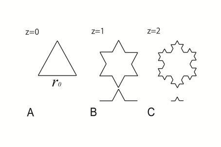
Von Koch fractal set

The sequential construction of the von Koch curve set begins with the initiator, which is an equilateral triangle of the side length r₀ (Fig. 1A). The iterated algorithm to generate the set of the von Koch curves (known as prefractals) is to recursively reduce the straight line segment (or the scale) by 1/3 exchanging repeatedly the middle third of each side of the initiator, or a preceding generator, with two sides of a smaller, equilateral triangle whose side is one-third the length of a previous side. The result after the first iteration (the stage of construction z = 1) is shown in Fig. 1B, and that after the second iteration (the stage of construction z = 2) in Fig. 1C. Continuation of this process results in the limit von Koch curve.

For the von Koch generators, the length of a segment at the z^th stage of construction (r_z) and the number of segments at the same stage (N_z) are, respectively,

, , (1)

where r₀ is the side length of the initiator (Fig. 1A). The length of the fractal curve, actually the perimeter since the curve is closed, (L_z), is defined as a product of the number of segments and the length of a segment, at the z^th stage of construction,

. (2)

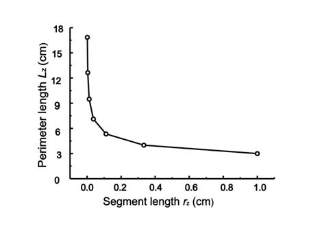
The inverse power law

From Eq. (2) it is evident that the perimeter of the von Koch prefractals diverges as z approaches infinity. If along the horizontal coordinate axis we put the values r_z = 1/3^z for z = 0,1,2,3, ... and along the vertical coordinate axis the values of L_z = 3·(4/3)^z also for z = 0,1,2,3, ..., and fit the power function to these data using Microsoft Excel software, the graph shown in Fig. 2 is obtained. The corresponding fitting parameters are also carried out and shown in

(3)

with the coefficients of determination R² = 1 and where r₀ = 1 cm for visual clarity. Generally, if we wish to express L as a function of r for similar fractal set, two constants of proportionality (α and β) should be used, thus the length can be written as

. (4)

The value β is the prefactor and α is the scaling exponent. From Eq. (3) it is seen that for the von Koch fractal set β = 3 and α = 0.262. We say that the length of a curve (a prefractal) scales with the length of the corresponding fractal segment. Or, mathematically, L_z is a unique function of r_z.

The simplest scaling relationship has the power law form [1]. The mathematical form of such scaling is an inverse power law scaling (Eq. (4)). It describes how a property L of the system (say a perimeter of the von Koch set) depends on the scale r at which it is measured [1]. Thus, this scaling relationship shows how the perimeter of a prefractal depends on the length of its segment: the smaller the length of the segment, the larger the perimeter. Since L= N·r (the expression known as the Richardson-Mandelbrot equation [20]), from Eq. (4) it follows that

(5)

Geometrical self-similarity

The object’s property known as self-similarity was first coined by Mandelbrot [7] and can be geometrical or statistical [1, 11, 24].

A fractal pattern is said to be geometrically self-similar if each small piece of it is an exact replica (i.e. ‘‘duplicate’’) of the whole object [1, 4]. Thus, the self-similarity qualitatively means that every small piece of an object resembles the whole object [1, 11]. This definition of the concept ‘geometrical self-similarity’ should be quantified since small pieces that constitute geometrical or natural objects are rarely identical copies of the whole object [22].

We have offered a more exact interpretation of this descriptive definition introducing a generating element of a generator as a “small piece” [5]. A generator is usually made up of straight-line segments (for instance, see Fig. 1). A particular and logical concatenation of some segments of a generator could be thought of as the generating element [11] of a generator if the whole object can be completely built with such elements by their translations and/or rotations.

In our example shown in Fig. 1 the generators of the von Koch prefractals, at the first and second stages of construction, have the generating elements made up of four equal segments each, as shown as details below the drawings in Fig. 1B and C. For example, the drawing in Fig. 1B can be subdivided into three generating elements, that in Fig. 1C into 12 elements, and so on.

Two generating elements of any two generators of a fractal set can be geometrically similar or not. According to the definition of similarity in Euclidean planimetry, two generating elements of the generators at stages z and z + 1 (say, those in Fig. 1B and C) are similar to each other if (a) the ratio of the measure of a segment of the generating element at stage z + 1 and the measure of the corresponding segment of the element at stage z is constant for all pairs of corresponding segments (e.g., for the four pairs of segments of the two mentioned details in Fig. 1) and for all z, and (b) the angles between the pairs of corresponding segments of the two generating elements are congruent. If the generating elements of the generators at stages z and z + 1 are similar for every z, we say that the whole class of the generators is geometrically self-similar, or, that this set has the property of geometrical self-similarity.

The similarity dimension

Mandelbrot [7] thinks that 'the plethora' of distinct definitions of the fractal dimension should be reduced to two: the similarity dimension and Hausdorff dimension. The similarity dimension (D_s) is basic dimension related to all self-similar (fractal) sets. We shall define this dimension using the von Koch set as an example. If all the scales of the prefractals at the stage of construction z are reduced by a factor F = 3, the number N_z ₊₁of the scales at the stage z + 1 becomes four times larger than at z. Indeed, since

(6)

it follows that

for every z. Generally, since N >F for every z, that fact can be presented by the expression

(7)

where D_s must be larger than 1. This relationship represents the definition of the similarity dimension D_s. This also can be presented as

(8)

For the von Koch set this dimension is D_s = log 4/log 3 = 1.262.

The Hausdorff dimension

One of the main differences between the methods of fractal geometry and fractal analysis is in treating the number N_z. In fractal geometry this value is the number of segments (scales) counted at z^thstage of construction carried out using the scale length r_z at the z^th stage of iteration. In fractal analysis this value, shown as N, represents the minimum number of the 'balls' of a given size (r) necessary to completely 'cover' the border (or a line) of an image. A ball consists of all points within a distance r from a center. In one dimension balls are line-segments, in two dimensions balls are circles, and in three dimensions balls are spheres. If one covers the object with balls of radius r it must be done so that every point of the object is enclosed within at least one ball. This may require that some of the balls overlap. One should find the minimum number of balls N(r) of size r needed to cover the object.

Consider the number N(r) of balls of radius at most r required to cover an object completely. When r is small, N(r) is large (similar relation exists between number of segments and scale length in fractal geometry). The Hausdorff dimension d is a number found such that N(r) grows with 1/r^d, as r approaches zero. The precise definition requires that the dimension d so defined is a critical boundary between the growth rates that are insufficient to cover the object, and the growth rates that are overabundant [18, 19]. The Hausdorff dimension d is theoretically rather complex but it is a successor to some less sophisticated but in practice very similar dimensions such as the capacity dimension.

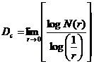
The modified capacity dimension

The similarity dimension can only be used to analyze geometrical (self-similar) fractal sets. Therefore, it would be necessary to generalize the similarity dimension. The most important results of such generalization are the Hausdorff and capacity dimension. These two dimensions are quite similar [1], but the Hausdorff dimension is rather sophisticated, being a subject of mathematical measure theory, and not suitable for practical use in fractal geometry. The capacity dimension is given by

(9)

It is suitable for determining irregularly shaped geometrical or natural objects. Since the logarithm is defined only for dimensionless values not for physical quantities like 1/r, we shall define the modified capacity dimension as

(10)

where r₀ is a reference scale [20, 21]. We will show that this quantity does not influence the common determination of the capacity dimension ((Eq. (9)). Such quantity r₀ ((Eq. (10)) is included into the definition of the capacity dimension, because the ratio r/r₀ is dimensionless quantity.

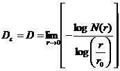
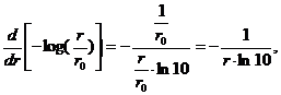
If we submit Eq. (5) into the last definition ((Eq. (10)) and put r , one can see that the expression in Eq. (10) represents an undetermined form, but nevertheless the limit of the quotient in Eq. (10) may exist. Application of the corresponding l'Hôpital's rule often converts an undetermined form to a determined one allowing easy evaluation of the limit. Let Q(r) = F(r)/G(r). Suppose, generally, that lim F(r) and lim G (r) when r . If these functions are differentiable on an open interval containing 0, il lim [F'(r)/G'(r)] exists and G'(r) 0 for all r from the interval, then

(11)

If the derivatives of F(r) = N(r) and G(r) = -log (r/r₀)

are inserted into Eq. (10), the limes of this expression (constant!) is

D = (12)

For the von Koch set D = 1.262 which is in accordance with the value obtained using the similarity dimension method. The expression given by Eq. (12) sometimes is presented as a definition of the fractal dimension: This statement is only a consequence of the definition given by Eq. (10). For that reason Eq. (5) may be presented as

(13)

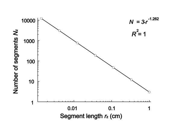
Equation (13) reveals as decreasing straight-line plots when the results of counting the numbers of segments are plotted on log–log axes against the values of the segment length. Thus if these data are presented in doubly logarithmic paper and fitted by a decreasing straight line, its coefficient of decreasing represents the fractal dimension D (Fig. 3). It should also be noticed that it will be wrong to enter the logarithms of the data into Descartes co-ordinate system, because, as we have noticed, logarithms of physical quantities have no physical sense.

Fractal dimension of biological objects

Unlike geometric fractal objects, biological and natural elements do express statistical self-similar patterns and fractal properties within an interval of scales, termed the ‘‘scaling window" [20]. It is defined experimentally by upper and lower limits in which a direct relationship between the observation scale and the measured size/length of the object or the frequency of a temporal event can be verified and in turn quantified by a peculiar D. The straight line fitting ceases out of the scaling limits to become a sigmoid curve with an asymptotic or even bi-asymptotic course, as revealed by several authors [26-29]. In other words, the measured dimensional parameters remain unaffected by further changes in resolution exceeding both limits. However, real ‘‘fractality’’ exists only when the experimental scaling range covers at least two orders of magnitude, although fractality over many orders of magnitude has been observed in various natural fields [30].

DISCUSSION

It is noticed before that geometrical self-similarity means that every small piece of an object resembles the whole object. Many authors tried to demonstrate graphically this definition [1, 4, 14]. We showed that such set of objects can be self-similar if their generating elements are geometrically similar. Any two prefractals of the von Koch set are not geometrically similar, contrary to their generating elements. This is obvious from Fig. 1B and C: these two images could only be visually alike, but not geometrically similar.

Losa and Nonnenchamer [20] used the expression N(ε) = l₀^D ε^-D, where ε is the unit length (corresponds to our r) and l_o is the reference scale. The value l₀^Dcorresponds to the prefactor β (Eq. (13)). It is important to notice that these authors underlined that β depended on D, which is not directly visible in the present study. Using this method they presented their dimensionless power law scaling.

Bassingthwaighte et al. [1] noted that the capacity dimension tell us how much balls needed to cover the object as the size of the balls (r) decreases. In the analytical definition of capacity dimension there exists log (1/r). West and Deering [11] defined the similarity dimension as the ratio of two logarithms ln N/ ln (1/r). In defining the box-counting dimension Falconer [18] showed lower and upper box-counting dimension by the expression containing log δ where δ is the diameter of a corresponding set. Edger [19] also use log (1/r) in the definition of the upper box-counting dimension, where r is a diameter of the set.

CONCLUSION

Since some concepts in fractal geometry are determined descriptively and/or qualitatively, this paper provides their exact mathematical definitions or explanations, and Richardson’s coastline method.

REFERENCES

1. Bassingthwaighte JB, Liebovitch LS, West BJ. Fractal physiology. New York & Oxford: Oxford University Press; 1994.

2. Smith TG, Lange GD, Marks WB. Fractal methods and results in cellular morphology – dimensions, lacunarity and multifractals. J Neurosci Meth. 1996;69:123–136.

3. Panico J, Sterling P. Retinal neurons and vessels are not fractal but space-filling. J Comp Neurol. 1995;361:479-490.

4. Fernández E, Jelinek HF. Use of fractal theory in neuroscience: methods, advantages, and potential problems. Methods 1998;24:9-18.

5. Ristanović D, Nedeljkov V, Stefanović BD, Milošević NT, Grgurević M, Štulić V. Fractal and nonfractal analysis of cell images: comparison and application to neuronal dendritic arborization. Biol Cybern. 2002;87:278-288.

6. Losa GA, Di Ieva A, Grizzi F, De Vico G. On the fractal nature of nervous cell system. Front.Neuroanat. 2011;5(45):1-2.

7. Mandelbrot BB. The fractal geometry of nature. NW Freeman and Co, New York: 1982.

8. Flook AG. Fractal dimensions: their evaluation and significance in stereological measurements. Acta Stereol. 1982;1:79-87.

9. Peng CK, Buldyrev SV, Goldberger AL, Havlin S et al. Long-range correlations in nucleotide sequences. Nature 1992;356:168-170.

10. Hoop B, Kazemi H, Liebovitch L. Rescaled range analysis of resting respiration. Chaos 1993;3:27-29.

11. West BJ, Deering W. Fractal physiology for physicists: Levi statistics. Phys Rep. 1994;246:1–100.

12. Caserta F, Eldred WD, Fernández E, Hausman RE, Stanford LR, Buldyrev SV, et al. Determination of fractal dimension of physiologically characterized neurons in two and three dimensions. J Neurosci Meth. 1995;56:133–144.

13. Bizzarri M, Giuliani A, Cucina A, Anselmi FD, Soto MA, Sonnenschein C. Fractal analysis in a system biology approach to cancer. Semin Cancer Biol. 2011; 21(3):175–182.

14. Thamrin C, Stern G, Frey U. Fractals for physicians. Paediatric Respiratory Rewiews 2010;11:123-131.

15. Perrotti V, Aprile G, Degidi M, Piattelli A, Iezzi G. Fractal analysis: a novel method to assess assess roughness organization of implant surface topography. Int J Periodontics Restorative Dent. 2011;31(6):633-639.

16. Tălu S. Fractal analysis of normal retinal vascular network. Oftalmologia. 2011;55(4):11-16.

17. Simon W. Mathematical techniques for physiology and medicine. Academic Press, New York and London 1972.

18. Falconer K. Fractal geometry. Mathematical foundations and applications. 2nd Edn. John Wiley and Sons, New York and London 2003.

19. Edger G. Measure, topology and fractal geometry. 2nd Edn. Springer, New York, 2008.

20. Losa GA, Nonnenmacher TF. Self-similarity and fractal irregularity in pathologic tissues. Mod Pathology 1996; 9 (3): 174-182.

21. Losa GA. Fractal morphology of cell complexity. Biology Forum, 2002; 95: 239-258.

22. Grizzi G, Ceva-Grimaldi G, Dioguardi N. Fractal geometry: a useful tool for quantifying irregular lesions in human liver biopsy specimens. J Anat Embriol. 2001;106 (Suppl.1):337-346.

23. Nakayama H, Kiatipattanasakul W, Nakamura S, Miyawaki K, Kikuta F et al. Fractal analysis of senile plaque observed in various animal species. Neurosci Lett. 2001;297:195-198.

24. Feder J. Fractals. New York: Plenum Press, 1998.

25. Losa GA. The fractal geometry of life. Theor Biol. 2009;102(1):29-59.

26. Paumgartner D, Losa GA, Weibel ER. Resolution effect on the stereological estimation of surface and volume and its interpretation in terms of fractal dimensions. J. Microsc. 1981; 121: 51–63.

27. Rigaut JP. An empirical formulation relating boundary length to resolution in specimens showing 'non-ideally fractal' dimensions. J. Microsc.1984; 13: 41–54.

28. Nonnenmacher TF, Baumann G, Barth A, Losa GA. Digital image analysis of self-similar cell profiles. J Biomed Comput. 1994; 37: 131–138.

29. Dollinger JW, Metzler R, Nonnenmacher TF. Bi-asymptotic fractals: fractals between lower and upper bounds. J Phys. A: Math Gen.1998; 31: 3839–3847.

30. Mandelbrot B. Is Nature fractal ? Science 1998; 279 (5352): 783–784.

LEGENDS TO FIGURES

Figure 1. Sequential construction of the von Koch curve set. (A) The initiator is the equilateral triangle of the side length r₀. (B) The first stage of construction (z = 1). (C) The second stage of construction (z = 2). Details below the drawings B and C represent the generating elements of the von Koch prefractals shown in B and C.

Figure 2. Hyperbolic decrease of the perimeters for the von Koch curves set. The perimeter (L_z ) of the von Koch prefractals plotted against the segment length (r_z).

Figure 3. Numbers of segments N_z shown on log-log axes against the length of a segment r_z. The graph is obtained using equation inscribed on the pictures. R² is the coefficient of determination.

FIGURE 1

FIGURE 2

FIGURE 3